Understanding OBIEE RPD - Chapter 1

Tweet

The most skilled task in the world of Oracle Business Intelligence is to design and code the RPD. While we are all aware of the general concepts of Business models, logical tables, joins and hierarchies, the RPD is essentially a query generating tool. The query generated by the tool depends on a sound understanding of the business model and data warehousing concepts. The most trickiest part of RPD development is to ensure that OBIEE generates a tuned physical query. I wish to write a series of articles that show the impact of coding something in the RPD on the Physical query and would hence enable the developers to find out the best things to do from a performance stand point. Please note that this article does not recommend one query over the other as the efficiency of the query will depend on the data structures themselves. The intention of this blog is to study the impact of changing the RPD on the Physical SQL.

This is the first article in this series and we will be talking about the scenario where we pull columns from 2 different physical sources and 1 common dimension in the same analysis.


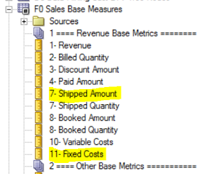
I selected the following columns

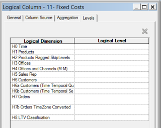
Let me now share the Aggregation rule and content level for both of the measure columns

So we see that none of the 2 measures are tagged to any level in the dimension and the aggregation rule is Sum.

Also note that both the measure columns are from the same logical fact.

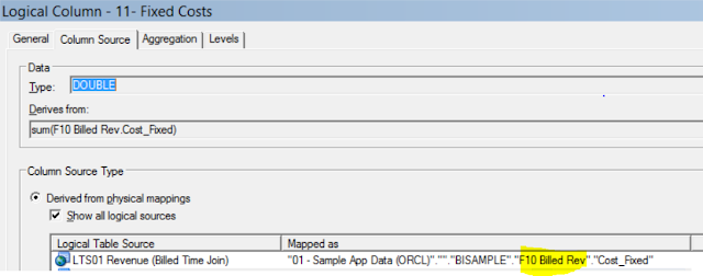
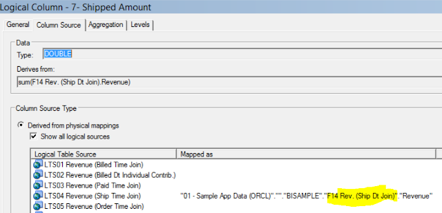
Let us now look at the column source mappings of each of these measures.

We note that these columns are mapped to different tables/aliases in the physical layer.

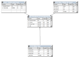
Let us now look at the physical layer joins of the tables involved in this Analysis.

Let us now look at the physical query generated by this analysis.

WITH 
SAWITH0 AS (select sum(T42433.Cost_Fixed) as c1,
     T42409.Prod_Dsc as c2,
     T42409.Prod_Key as c3
from 
     BISAMPLE.SAMP_PRODUCTS_D T42409 /* D10 Product (Dynamic Table) */ ,
     BISAMPLE.SAMP_REVENUE_F T42433 /* F10 Billed Rev */ 
where  ( T42409.Prod_Key = T42433.Prod_Key ) 
group by T42409.Prod_Dsc, T42409.Prod_Key),
SAWITH1 AS (select sum(T68770.Revenue) as c1,
     T42409.Prod_Dsc as c2,
     T42409.Prod_Key as c3
from 
     BISAMPLE.SAMP_PRODUCTS_D T42409 /* D10 Product (Dynamic Table) */ ,
     BISAMPLE.SAMP_REVENUE_F T68770 /* F14 Rev. (Ship Dt Join) */ 
where  ( T42409.Prod_Key = T68770.Prod_Key ) 
group by T42409.Prod_Dsc, T42409.Prod_Key),
SAWITH2 AS (select D1.c1 as c1,
     D1.c2 as c2,
     D1.c3 as c3,
     D1.c4 as c4,
     D1.c5 as c5
from 
     (select 0 as c1,
               case  when D1.c2 is not null then D1.c2 when D2.c2 is not null then D2.c2 end  as c2,
               D1.c1 as c3,
               D2.c1 as c4,
               case  when D1.c3 is not null then D1.c3 when D2.c3 is not null then D2.c3 end  as c5,
               ROW_NUMBER() OVER (PARTITION BY case  when D1.c2 is not null then D1.c2 when D2.c2 is not null then D2.c2 end , case  when D1.c3 is not null then D1.c3 when D2.c3 is not null then D2.c3 end  ORDER BY case  when D1.c2 is not null then D1.c2 when D2.c2 is not null then D2.c2 end  ASC, case  when D1.c3 is not null then D1.c3 when D2.c3 is not null then D2.c3 end  ASC) as c6
          from 
               SAWITH0 D1 full outer join SAWITH1 D2 On D1.c3 = D2.c3
     ) D1
where  ( D1.c6 = 1 ) )
select D1.c1 as c1, D1.c2 as c2, D1.c3 as c3, D1.c4 as c4 from ( select D1.c1 as c1,
     D1.c2 as c2,
     D1.c3 as c3,
     D1.c4 as c4
from 
     SAWITH2 D1
order by c1, c2 ) D1 where rownum <= 5000001

Lesson: We see that we have 2 with clauses joined by a full outer join. This is primarily because F10 Billed Rev and F14 Rev. (Ship Dt Join) are 2 LTS in the same Logical table. Since these LTS are not joined in the Logical table so these should essentially be calculated separately. However, the analysis demands that these be joined together. So what does OBIEE do? It calculates them separately and then joins them using a Full Outer Join.

Let us now join F10 Billed Rev and F14 Rev. (Ship Dt Join) in the physical layer and then join them in a single LTS as shown below.

Let us now look at the Business model and the generated query.

WITH 
SAWITH0 AS (select sum(T286916.Units) as c1,
     sum(T286892.Cost_Fixed) as c2,
     T286942.Prod_Dsc as c3
from 
     SAMP_PRODUCTS_D T286942 /* D10 Product (Dynamic Table) */ ,
     SAMP_REVENUE_F T286892 /* F10 Billed Rev */ ,
     SAMP_REVENUE_F T286916 /* F14 Rev. (Ship Dt Join) */ 
where  ( T286892.Bill_Qtr_Key = T286916.Bill_Qtr_Key and T286892.Cust_Key = T286916.Cust_Key and T286892.Order_Key = T286916.Order_Key and T286892.Prod_Key = T286916.Prod_Key and T286892.Prod_Key = T286942.Prod_Key and T286892.Empl_Key = T286916.Empl_Key and T286892.Bill_Mth_Key = T286916.Bill_Mth_Key and T286892.Shipto_Addr_Key = T286916.Shipto_Addr_Key and T286892.Office_Key = T286916.Office_Key and T286916.Prod_Key = T286942.Prod_Key ) 
group by T286942.Prod_Dsc)
select D1.c1 as c1, D1.c2 as c2, D1.c3 as c3, D1.c4 as c4 from ( select distinct 0 as c1,
     D1.c3 as c2,
     D1.c2 as c3,
     D1.c1 as c4
from 
     SAWITH0 D1
order by c2 ) D1 where rownum <= 5000001

Moral of the Story:

1. This join is a Fact to Fact join. This is not advisable from a datawarehouse modelling perspective but it results in improved query in certain cases. 

2. The implications of this join on other Analysis should be thought out well before implementing the same. There might be some other analysis in which you might not want to follow the old access path.

Let us now bring in the 2 fact sources as separate Logical tables in the BMM and see the result. Let me share the new BMM model

Note that F10 Billed Rev and F14 Rev. (Ship Dt Join) are separate Logical tables in the BMM.

The resulting query is

WITH 
SAWITH0 AS (select sum(T286892.Cost_Fixed) as c1,
     T286942.Prod_Dsc as c2
from 
     SAMP_PRODUCTS_D T286942 /* D10 Product (Dynamic Table) */ ,
     SAMP_REVENUE_F T286892 /* F10 Billed Rev */ 
where  ( T286892.Prod_Key = T286942.Prod_Key ) 
group by T286942.Prod_Dsc),
SAWITH1 AS (select sum(T286916.Units) as c1,
     T286942.Prod_Dsc as c2
from 
     SAMP_PRODUCTS_D T286942 /* D10 Product (Dynamic Table) */ ,
     SAMP_REVENUE_F T286916 /* F14 Rev. (Ship Dt Join) */ 
where  ( T286916.Prod_Key = T286942.Prod_Key ) 
group by T286942.Prod_Dsc),
SAWITH2 AS (select D1.c1 as c1,
     D1.c2 as c2,
     D1.c3 as c3,
     D1.c4 as c4
from 
     (select 0 as c1,
               case  when D1.c2 is not null then D1.c2 when D2.c2 is not null then D2.c2 end  as c2,
               D1.c1 as c3,
               D2.c1 as c4,
               ROW_NUMBER() OVER (PARTITION BY case  when D1.c2 is not null then D1.c2 when D2.c2 is not null then D2.c2 end  ORDER BY case  when D1.c2 is not null then D1.c2 when D2.c2 is not null then D2.c2 end  ASC) as c5
          from 
               SAWITH0 D1 full outer join SAWITH1 D2 On D1.c2 = D2.c2
     ) D1
where  ( D1.c5 = 1 ) )
select D1.c1 as c1, D1.c2 as c2, D1.c3 as c3, D1.c4 as c4 from ( select D1.c1 as c1,
     D1.c2 as c2,
     D1.c3 as c3,
     D1.c4 as c4
from 
     SAWITH2 D1
order by c1, c2 ) D1 where rownum <= 5000001

We see that the query is the same as that in the 1st case where we did not have the join. The reason? We don't have a join in the Business model between the 2 fact sources. So the BI server does not use the join between these sources in the Physical layer.

I know what you are thinking. Why dont we join the 2 fact sources in the BMM? Well, in this case, SAMP_REVENUE_F is the source of both F10 Billed Rev and F14 Rev. (Ship Dt Join). So the join should ideally have a 1 to 1 cardinality. Now, joining with this cardinality will result in circular join.

Many to Many join does not make sense in this scenario but let's say we did it, we will have to introduce a bridge table to fulfil the join. The last option is to make one tabe as fact and the other as dimension but this will cause the measure from the table acting as dimension to become null and void. OBIEE will not display this measure because measures cant be in dimensions.

The logical SQL will be

SELECT
   0 s_0,
   "Vishal"."Products"."P1  Product" s_1,
   "Vishal"."F10 Billed Rev"."11- Fixed Costs" s_2,
   "Vishal"."F14 Rev. (Ship Dt Join)"."7- Shipped Amount" s_3
FROM "Vishal"
ORDER BY 1, 2 ASC NULLS LAST
FETCH FIRST 5000001 ROWS ONLY

and the physical SQL will be

WITH 
SAWITH0 AS (select sum(T286916.Units) as c1,
     T286942.Prod_Dsc as c2
from 
     SAMP_PRODUCTS_D T286942 /* D10 Product (Dynamic Table) */ ,
     SAMP_REVENUE_F T286916 /* F14 Rev. (Ship Dt Join) */ 
where  ( T286916.Prod_Key = T286942.Prod_Key ) 
group by T286942.Prod_Dsc)
select D1.c1 as c1, D1.c2 as c2, D1.c3 as c3, D1.c4 as c4 from ( select distinct 0 as c1,
     D1.c2 as c2,
     cast(NULL as  DOUBLE PRECISION  ) as c3,
     D1.c1 as c4
from 
     SAWITH0 D1
order by c2 ) D1 where rownum <= 5000001

Here, F10 Billed Rev was acting as the dimension. You will also see the following error in your logs

Expression '11- Fixed Costs:[DAggr(F10 Billed Rev.11- Fixed Costs by [ D1 Products (Level Based Hier).P1  Product] )]' converted to NULL because [nQSError: 14020] None of the fact tables are compatible with the query request 11- Fixed Costs:[DAggr(F10 Billed Rev.11- Fixed Costs by [ D1 Products (Level Based Hier).P1  Product] )]

Till next time ..